Artificial intelligence for automatic phase identification in powder X-ray diffraction

X-ray diffraction represents a powerful tool for identification of unknown powder phases [Mittemeijer, E. J. & Scardi, P. (eds.) (2004). Diraction Analysis of the Microstructure of Materials, vol. 68 of Springer Series in Materials Science. Springer; Cleareld, A., Reibenspies, J. & Bhuvanesh, N. (eds.) (2008). Principles and Applications of Powder Diffraction. Wiley-Blackwell]. This procedure is commonly performed by matching the measured pattern with a reference database. The best candidate phases are chosen according to some measure of their similarity to the measured data and quantified by a figure of merit (FOM). Standard strategy of FOM calculation (see e.g. [Altomare, A. et al. J. Appl. Cryst., 2015, 48, 598; Altomare, A. et al. J. Appl. Cryst., 2008, 41, 815]) is to combine several similarity criteria (correspondence of peaks positions, intensities, etc.) so that candidates ranking is performed according to certain requirements. This approach, being quite natural as an algorithmization of manual search technique, becomes less clear when modifications and adaptation for problems, not supported by our intuition, are required (accounting for coinciding peaks of several phases, “additive” search, solid solutions, etc.). Even more difficulties are encountered, when systematic errors, affecting multiple peaks in a correlated and reproducible way, are present. Such errors may hinder the correct identification of phases even when they are relatively small.

If one is trying to design an approach suitable for fully automatic powder phase identification, a number of questions arise. Can the search and match strategy be formulated in the way, suitable for modification and adaptation without applying to scientists' intuition and experience? Can the phase identification procedure be derived from certain basic physical assumptions, rather than stated in its final form?

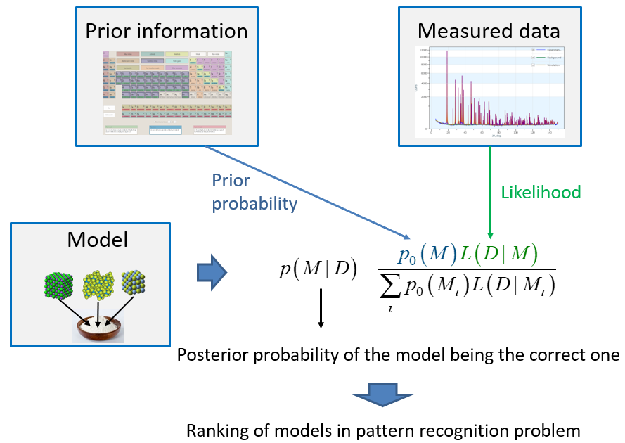
The research, conducted by Atomicus team, enabled us to give positive answers to both questions. We found physically grounded expressions for FOM calculation on the basis of Bayes’ rule, which has already been accepted as a powerful approach for measured data patterns analysis [Gilmore C. J. Acta Cryst., 1996, A52, 561; David, W. I. F. and Sivia, D. S. J. Appl. Cryst., 2001, 34, 318; Bergmann, J. and Monecke, T. J. Appl. Cryst., 2011, 44, 13; Mikhalychev, A. et al. Phys. Rev. A, 2015, 92, 052106]. The approach is schematically shown in Figure 1. The a priori information, if available, can be introduced by modifying the prior probabilities of different phases or chemical elements. The correspondence between the measured and the reference patterns is quantified by the likelihood function, which takes into account a model (probability distribution) of the possible experimental inaccuracies. An important complication of the patterns analysis is imposed by the fact that a realistic sample contains multiple phases, their patterns forming the measured spectrum together. To calculate the FOM for a given candidate phase, we take into account not only the likelihood of the difference between the reference and the observed (formed by the matched peaks) patterns of the phase, but also the estimated probability of explaining the rest of the spectrum by other phases.

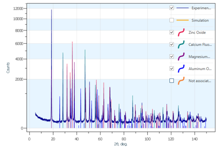
The approach can include any desired level of physical detailing in prior probabilities specification and is applicable for multi-phase samples with coinciding peaks, for calculation of “collective” FOM for a combination of several reference substances, for stable and justified finding intensity scales (for subsequent quantitative analysis). It combines universality with high performance and is suitable for implementation of an artificial intelligence-based assistant, which is capable of fast and accurate guiding of an analyst through the phase identification process. The approach has been applied to IUCr round robin examples [www.iucr.org/resources/commissions/powder-diffraction/projects/qarr] and demonstrated correct identification of all the phases (see an example in Figure 2).

If the peak pattern has a systematic peak shift, ignoring this systematic error can lead either to miss of the correct phases (for a small tolerance window) or to multiple false hits (for a large window). On the other hand, strong correlation of peak shifts, caused by the systematic errors, leaves the possibility of their detection and correction. To address the problem, we updated our initial artificial intelligence approach to make it applicable to the case when both random and systematic errors are present. The a priori assumptions about the error probabilities are used to estimate the posterior probabilities of the phases’ presence in the investigated sample. On acceptance of each new phase by the operator, the modified algorithm learns more about the probable systematic errors by updating corresponding probability distributions. Figure 3 shows application of the algorithm to the data with artificially introduced specimen displacement errors. The results clearly show advantages of the proposed modification of the approach, which made it capable of automatic detection and correction of systematic errors without any necessity of additional actions of the operator.

The results (the initial version of the approach before its modification) are published in the following paper: Mikhalychev, A. and Ulyanenkov, A. J. Appl. Cryst. 2017, 50, 776-786. (https://scripts.iucr.org/cgi-bin/paper?rg5114, www.researchgate.net)